Case Study: Brand Name Change

The company recently changed its brand name and knowledge of the effect of the rebranding on the customers perceived satisfaction with its products is necessary. Customer Satisfaction is a significant performance indicator for any company or organization (Fornell, Rust, & Dekimpe, 2008). Customer Satisfaction is often considered a latent variable usually measured using a survey with a set of questions. A company may want to know how a change affects the perceptions of consumers. Consequently, a single variable or multiple variables relating to the customer satisfaction can be measured (Montinaro and Chirico, 2006). In most cases, variables of the satisfaction domain are on ordinal scale with various levels of categories binary or Likert scale with several modalities and scores, etc. to indicate the levels of satisfaction.

Different approaches to the analysis of this kind of data can be found in the literature. Manisera (2007) explored the priori quantification of each ordinal variable before applying multivariate methods. Lauro et al. (2011) and Tenenhaus and colleagues (2005) explained the approach by estimating the scores of qualitative variables within iterative methods of statistical estimation. Other approaches to data analysis include latent variables with ordinal variables (Cagnone and Mignani, 2009; Moustaki, 2000; Moustaki, Joreskog, & Mavridis, 2004; Winship & Mare, 1984), Rasch Analysis (Duncan et al., 2003; Tesio, 2003), and stochastic models for ordinal variables (Agresti & Kateri, 2011; McCullagh, 1980; Tijms, 1994).

The present study is a correlational study where data were collected before and after the brand name change. For this study, a simple random sampling was used to select participants for the study. Every shopper had an equal chance of being chosen for the 20 items identified to examine the change in the satisfaction of consumers after brand name change. Simple random sampling is one of the gold standards of probability sampling in that the technique reduces the risk of bias in the selection of subjects to be included in the study. Consequently, this sampling method provides the researcher with a highly representative sample of the population under study, the assumption being limited missing data. The probabilistic method used in the selection of simple random sample makes it possible for the researcher to generalize the sample to the population (or statistical inference). As a result, the generalizability of a sample of the population is considered as having external validity.

The sample of the present study included customers of the company who bought select 20 items. These products are a random sample representing their average customer satisfaction. As stated above, the sample is a random representation of the companys customers where each customer was given an equal chance of partaking in the study. The outcome of the survey would then be statistically inferred to the entire consumer base.

To determine whether changing the brand name actually had an impact on consumer satisfaction, it was necessary to measure the satisfaction levels before and after the brand name change. In this case, satisfaction scores after the rebranding are dependent upon the satisfaction scores before alteration of the brand name. Therefore, the scores before represent the independent variable while the scores after are the dependent (predictor) variable. In this study, the items under investigation (e.g. Headsets, Speakers, CD player, and Alarm Clock, etc.) are our nominal values. Typically, nominal values are not calculated because they just represent an approximation or an accepted condition rather than a real value. However, the satisfaction scores before and after the brand name change are real values that are represented as scale values or ratios. There are no confounding, lurking, or missing variables that have not been included in the case study.

The results of the study were recorded in Table 1 as follows;

Table 1:

Summary of raw customer satisfaction data before and after change

Product Customer

Satisfaction

Rating (before) Customer

Satisfaction

Rating (after)

Headset A 2.4 2.7

Speakers 8.9 7.6

CD Player 5 6

DVD Player 7.2 7.1

Alarm Clock 9 8.4

Stereo 8.8 8.6

Shower Radio 7.7 7.7

Surround System 6.1 6.0

Satellite Radio 6.3 5.9

Microphone 4.3 8.2

Bluetooth Speakers 1.1 3.4

Karaoke System 2.6 3.5

Earbuds 7.2 7.5

Gaming Headset 8 8.9

Expanding Speaker 5.1 6.2

Portable Speaker 7.9 7.6

Multimedia Speaker 5.6 5.7

Phone Charger 5.2 5.3

Wireless headphones 6.4 7.8

Portable Keyboard 8.2 8.1

This data was entered into MS Excel workbook and SPSS for both descriptive and inferential analysis.

Primary Data Analysis

Examination of Descriptive Statistics

Descriptive statistics are useful in helping us understand complex data in a simpler way. Raw data such as in Table 1 above can be hard to visualize, especially if there is a lot of it. The role of descriptive statistics is, therefore, to enable us to understand in a much simpler way complex data. These statistics are performed in the form of univariate analysis, which involves examination of the distribution, the central tendency, and dispersion. In the present study, only measures of central tendency and dispersion were examined for the primary data. Table 2 provides a summary of these measures of central tendency mean, mode, and median values) and measures of dispersion (standard deviation, variance, and range).

Table 2.

Summary of Descriptive Statistics

N Range Mean Median Mode SD Variance

Satisfaction (Before) 20 7.90 6.15 6.35 7.20 2.26309 5.122

Satisfaction (After) 20 6.20 6.61 7.30 6.00 1.80610 3.262

Valid N (listwise) 20 Central Tendency

The average satisfaction scores before the brand name change were 6.15 (SD = 2.26309) while those of satisfaction after was 6.61 (SD = 1.80610). This data shows that the means of before and after scores are not the same, i.e., at face value, there has been a change. The average score is the most frequently used measure of central tendency, but it is also sensitive to extreme scores. An alternative statistic to mean is median. The advantage of using median is that it is not sensitive to extreme scores (outliers) and can, therefore, be used where mean is unable to be used due to the presence of outliers. In Table 2, the median value of Satisfaction Scores (Before) was 6.35, and that of Satisfaction (After) was 7.30. This implies that half of the scores were 6.35 and below while the other half of the Satisfaction Scores (Before) were 6.35 and above. Similarly, half of the Satisfaction (After) scores were 7.30 and below, while the second half was 7.30 and above. Mode refers to the most common value present in a set of data. It does not involve any calculation or ordering of data to find the mode value. In our data, 7.20 were the mode value for the first set of data (Satisfaction Before scores) and 6.00 for the Satisfaction (After) scores. The Mode is often used with categorical data more than it is used with other types of data.

Distribution

In real life situations, most variables tend to be normally distributed. This can be represented as normal distribution curve (normality curves), which is dome shaped and symmetrical about the mean. On the normal distribution curve, all the measures of central tendency i.e. the mean, median, and mode are all equal. In other words, the normal distribution curve is a function of the average and standard deviation. There are variations or spread of distributions for various sets of data. Range and standard deviation are values that are often associated with this spread of the distribution. Range value represents a comparison between the minimum and maximum satisfaction scores in this study. It is the difference between the maximum and the minimum score. For Satisfaction Before scores, the difference between the highest and lowest value (range) is 7.90 (See Table 2). Similarly, the range value for the Satisfaction After score is 6.20 (Table 2). These range values are estimates of the variation of the satisfaction scores because it does not indicate much how much the satisfaction values/ scores vary from the average scores and about the shape of the distribution curve.

Another increasingly important variable that shows a lot about the distribution of our data is the standard deviation. The standard deviation is indicative of what is going on between the lowest and the highest satisfaction scores. In fact, the standard deviation is telling us how much the customer satisfaction scores in the data set vary around the mean. As such, the standard deviation was useful in comparing the Satisfaction "Before" and Satisfaction "After" scores using the same scale.

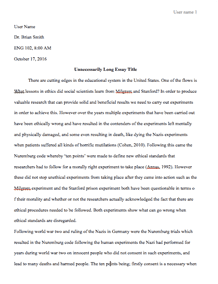
Figure 1: Normal distribution curve of Satisfaction Before scores. A distribution curve has been superimposed on the histogram. The curve is not multimodal, asymmetric, and negatively skewed. Half of the satisfaction ratings (Before) should be above the mean (M = 6.15) in a perfect normal distribution curve. The variance of Satisfaction Before scores is 5.122, which tells us about how far the satisfaction scores are spread out. The higher the difference value, the larger the spread from the mean. A lower variance value would represent a clustering of the scores around the average.

Figure 2. Normal distribution curve of Satisfaction After scores. This distribution curve is similar to that in Figure 1. The curve is not multimodal, asymmetric, and negatively skewed. Half of the satisfaction ratings (After) should be above the mean (M = 6.61) in a perfect normal distribution curve. However, most of the satisfaction scores in this study fall towards the higher side of the scale. In some cases, data is transformed to obtain the normal distribution. The variance of Satisfaction Before scores is 5.122, which tells us about how far the satisfaction scores are spread out. The higher the variance value, the larger the spread from the mean. A lower variance value would represent a clustering of the scores around the average.

Skewness in statistics is a measure of the asymmetry of distribution of random variables around the average score. The probability skewness value can be positive (concentrated on the lower side) or negative (concentrated on the higher side). A distribution curve plays a significant role in telling us whether the distribution of scores is symmetric or asymmetric. Besides, it shows the type of skewness of the skewed distribution.

Examination of Inferential Statistics

A correlation analysis was conducted to determine the effects of the brand name change on customer satisfaction scores.

Paired t-test

The study was guided by the following: Is there a difference between the Satisfaction Before scores and Satisfaction After scores following the brand name change?

The paired t-tests were performed to compare the means of data from the two groups (related samples). The satisfaction scores before and after changing the brand name are recorded in Table 1. Satisfaction scores are scale data that are often summarized by calculating the average and standard deviation (SD). The paired t-test is used to compare the means of the two samples of related data on the same set of participants. The paired t-test compares the difference of average values to zero, and it is influenced by the difference in mean, the number of data, and variances of mean differences.

The Satisfaction Before scores were used as the independent (predictor) variables and the Satisfaction After scores used as the dependent variables.

Assumption #1: The first assumption was that the dependent variable is continuous i.e. measured at interval or ratio level. The scale variab...