Exploring the Incidence of Disruptive Status in Two Groups of People: With ADHD and Without ADHD

Young, Gudjonsson, Ball and Lam (2003) used the independent t-test of hypothesis of a mean difference to test their research hypothesis. The independent t-test assumes that, in an analysis, the variables are categorized as either independent or dependent. With variables falling in either the independent or the dependent category, it means the differences in the mean score of the dependent variable results from the variation in the independent variable. The independent samples t-test deals with samples that do not have a relationship with each other; for these samples, the selection of a subject for inclusion into the sample does not affect the selection of another subject for inclusion into the same sample. In Young et al. (2003)s study, the independent samples t-test was appropriate because the variables that the researchers were examining could be considered either dependent or independent. The researchers were exploring the incidence of disruptive status in two groups of people people with attention deficit hyperactivity disorder (ADHD) and those without ADHD.

The independent variable in Young et al. (2003)s study was ADHD, while the dependent variable was disruptive status; the difference in the participants disruptive status resulted from the extent to which they were suffering from ADHD. In addition, the two samples used in Young et al. (2003)s study were independent because the categorization of a participant as one who is suffering from ADHD did not affect the assignment of another participant into the non-ADHD group. Overall, the independent samples t-test was appropriate for the study by Young et al. (2003). However, there were certain limitations of using the independent samples t-test in Young et al. (2003)s study. One assumption of the independent samples t-test is that the variance of the two samples is homogenous. Looking at the findings in Young et al. (2003), it is apparent that there was a violation of the assumption of homogeneity of variances. The standard deviation of the scores of the participants in the non-ADHD group (14.59, 10.58 and 7.01) was different from the standard deviation of the scores in the ADHD group (16.44, 13.77, and 7.08), and this shows that the two samples did not have the same variance.

The standard deviation of the scores on critical incidents, too, was not the same in the ADHD group and the non-ADHD group. Fortunately, for the non-ADHD group, the violation of the assumption of homogenous variances did not have a serious effect on the tests robustness. According to the Central Limit Theorem, as long as samples are large enough (comprising at least 30 subjects), violations of the assumption of homogeneity of variances do not affect the validity of statistical tests (Brase and Brase, 2017). The non-ADHD group had 46 subjects, and this means that the violation of the assumption of homogeneity of variance did not affect the validity of the independent t test in this group. The problem is in the ADHD group that comprised 23 subjects a sample size lower than the size required to keep statistical tests robust despite violations.

The low birth-weight data set (herein referred to as the data set) shows data on infants at birth, including the age of the mother, the race of the mother, whether the mother smokes, and the infants weight. The age of the mother has been measured at the interval level, and so has the infants birth weight; this indicates that these two variables are quantitative. The other two variables the race of the infants mother and the smoking status of the infants mother have been measured at the nominal level, suggesting that these variables are qualitative. In this paper, the low birth-weight data is used to test three hypotheses.

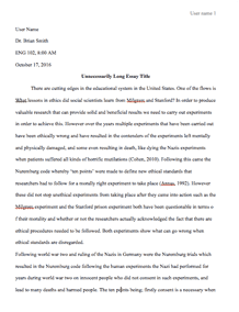
The first hypothesis is that the mothers smoking status influences an infants birth weight. Stated in the null form, the first hypothesis is that the mothers smoking status does not influence an infants birth weight. If a mothers smoking status does not influence an infants birth weight, then one should not expect a difference between the birth weight of an infant whose mother smokes and the birth weight of an infant whose mother does not smoke. To test the first hypothesis, this paper uses the independent t-test of hypothesis of the mean difference. The following table summarizes the birth weight for infants in two groups the infants whose mothers smoke and the infants whose mothers do not smoke.

Table 1: Smoking status and birth weight

Group Statistics

Mother's smoking status N Mean Std. Deviation Std. Error Mean

Infant's birthweight does not smoke 115 3054.96 752.409 70.163

smokes 74 2773.24 660.075 76.732

From table 1, it is apparent that the mean for the group whose mothers do not smoke is higher than the mean for the group whose mothers smoke. Table 2 below shows the SPSS results for the independent t-test of hypothesis.

Table 2: Independent samples t test

Independent Samples Test

Levene's Test for Equality of Variances t-test for Equality of Means

F Sig. t df Sig. (2-tailed) Mean Difference Std. Error Difference 95% Confidence Interval of the Difference

Lower Upper

Infant's birthweight Equal variances assumed 1.508 .221 2.634 187 .009 281.713 106.969 70.693 492.734

Equal variances not assumed 2.709 170.001 .007 281.713 103.974 76.467 486.960

The null hypothesis was that mean weight in the two groups is the same, and this paper tests this hypothesis at a 5% significance level. The 5% (0.05) significance level means that, if the null hypothesis were true, there is at least a 5% chance of observing a t-test statistic as large as the one that one gets from the data set. In table 2, assuming that the two groups have the same variance, there is a 0.9% chance (0.009 sig. level) of observing a t-test statistic as large as the one that the data set gives. Therefore, if there is no difference in the mean of the group of infants whose mothers smoke and the mean of the group of infants whose mothers do not smoke, it is highly unlikely that the data set would give a t-test statistic of 2.634. Considering the outcome of the independent t-test, there is insufficient evidence to support the null hypothesis, and this paper rejects that hypothesis. In conclusion, there is a significant difference in the mean of the two groups, and this suggests that smoking status influence the birth weight of infants. The limitation of using the independent t-test in evaluating the influence of smoking status on the infants birth weight is that the two groups smoking mothers and non-smoking mothers - do not have the same size, and this can potentially reduce the validity of the independent t-test in exploring the influence of smoking status on the infants birth weight.

The second hypothesis that this paper tested using the data set is that race influences the birth weight of infants. Stated in the null form, the hypothesis is that the mean birth weight of infants is the same in the three races white, black, and Asian American. The alternative hypothesis is that the mean birth weight of infants is different across the three races. Considering that in the second hypothesis, this paper is comparing three groups, the F-test of hypothesis for mean differences is the most appropriate for testing the null hypothesis. Table 3 below shows the results of the one-factor ANOVA that was used in computing the F ratio.

Table 3: F-test of mean differences

ANOVA

Infant's birthweight Sum of Squares df Mean Square F Sig.

Between Groups 5070607.632 2 2535303.816 4.972 .008

Within Groups 9.485E7 186 509927.124 Total 9.992E7 188

In table 3, the variation between groups is compared to the variation within groups to get the F ratio. This paper tests the null hypothesis at the 5% (0.05) significance level; this means that, if the mean birth weight is not different across the three racial groups, there is at least a 5% chance of observing an F ratio as large as the one that the data set gives. From table 3, the F ratio has a significance value of 0.008 (0.8%), and this suggests that, if the null hypothesis is true, there is a 0.8% chance of getting an F ratio of 4.972 from the data set. Therefore, if the null hypothesis is true, it is highly unlikely that one would get the data that the author of this paper did, suggesting that there is insufficient evidence to support the null hypothesis. In conclusion, the mean birth weight differs across the black, white and Asian American races, and this means that race could be a significant factor influencing an infants birth weight. The F-test of hypothesis for mean differences assumes that the variance in the groups under comparison is homogenous (Bryman, 2015; Ott and Longnecker, 2015). However, in this case, the three groups under comparison did not have the same variance. The violation of the assumption of homogeneity of variances introduces one limitation of using the F-test to test the second hypothesis: the test may not be valid considering some of the conditions required for its validity were absent. Fortunately, the F-test seems robust to violations of some assumptions (Jackson, 2015).

The third hypothesis that this paper tests using the data set is that the age of an infants mother can predict that infants birth weight. Stated in the null form, the hypothesis is that a mothers age does not predict the birth weight of an infant. Considering that simple regression analysis helps in predicting the value of one variable from the value of another variable, this paper employs it to test the third hypothesis. Table 4 below shows the summary of the regression of the infants birth weight on the mothers age.

Table 4: Regression model summary

Model Summary

Model R R Square Adjusted R Square Std. Error of the Estimate

1 .090a .008 .003 728.011

a. Predictors: (Constant), Mother's age From table 4, R - the coefficient of correlation is 0.09, and this shows that the correlation between the mothers age and an infants birth weight is low. The R Square - the coefficient of determination - is 0.008, and this suggests that about 0.8% of the variation in the infants birth weight results from the variation in their mothers ages. Table 5 below shows the results test of the significance of the regression model.

Table 5: Test of significance of regression model

ANOVAb

Model Sum of Squares df Mean Square F Sig.

1 Regression 806926.913 1 806926.913 1.523 .219a

Residual 9.911E7 187 530000.672 Total 9.992E7 188 a. Predictors: (Constant), Mother's age b. Dependent Variable: Infant's birthweight In this paper, the F-test of significance of a regression model was used to test the hypothesis that the age of the mother significantly predicts an infants birth weight. The F-test compares the regression sum of squares to the residual sum of squares, and, therefore, shows if the variation that a regression model explains is more than the variation that the model does not explain. The simple regression model was tested at significance at the 0.05 level; this means that, if indeed the mothers age does not predict the infants birth weight, there is at least a 5% chance of observing an F-ratio as large as the one that one gets from the mothers age and infants birth weight data. Looking at table 5, the F-ratio has a significance value of 0.219, and this means that if the regression model does not predict the infants birth weight, there is a 21.9% chance that one would get a data set (like the one in this case) that gives an F-ratio of 1.523. The findings indicate that if the mothers age does not predict the birth weight of an infant, there is a high probability that one would make observations conforming to the data set in this paper. Therefore, there is enough evidence to support the hypothesis that the regression model does...